Uninformed Search Part 1


By Brian Williams, Viraj Parimi, Alisha Fong, and Cameron Pittman. It takes approximately 1 hour to complete this lesson.
Our agent will need to select specific actions and maneuvers from a large set of possibilities. In effect, it needs to decide what to do and when to do it. Search algorithms are necessary components for answering both questions. Uninformed search, or "blind" search, forms the basis on which more advanced search algorithms are built. The goal of this lesson is to make the abstract idea of search concrete by giving you hands on experience implementing two blind search algorithms, Depth-First Search and Breadth-First Search.
Imagine being given a box of Legos with no instructions and being tasked to build a car. There may not even been a correct answer. There's a large, but finite number of bricks. They only fit together in specific orientations. How would you go about building the car?
 Maybe the box looks like this? Source.
Regardless of the way the car looks or the types of components, you'll have to systematically compare bricks and their combinations to work towards something that resembles a car.
A state-space search is one way to frame the systematic approach to finding the right pieces and combinations. In this lesson, we'll dive into what it means to perform a state-space search, look at depth-first search and breadth-first search as two algorithms, and then you'll implement both algorithms to solve a simpler problem (compared to building a Lego car) called the 8-Tile Puzzle.
State-Space Search
A decision problem is framed by three things: 1) a set of inputs, 2) a set of outputs, and 3) a correct mapping between inputs and outputs.
The input to a state-space search problem is a graph with a start and a goal. The output is a path from the start to the gaol.
Graphs and Inputs
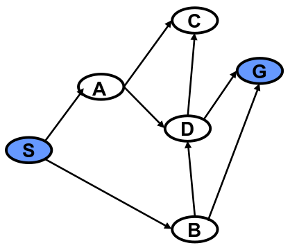
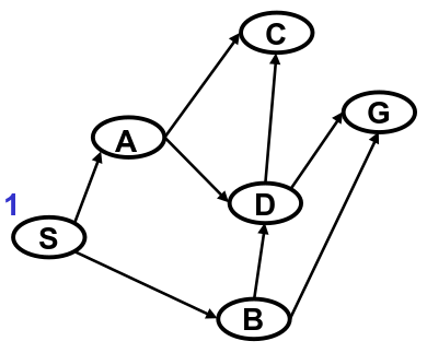
Graphs are data structures like the one you see above. They consist of vertices (or nodes), which in our case are represented by circled letters. The black arrows between the vertices represent edges.
In mathematical shorthand, we refer to the graph as , the set of all vertices as , and the set of all edges as . The vertex that represents the starting state is called , and the vertex that represents the goal state is . (Capitalization is important! and do not represent the same thing!).
The vertices of denote the states of the problem, and its edges, , denote the operators of the problem.
Output
The output of a state space search problem is a path (or sequence) of vertices, , in . Not all sequences of vertices are valid solutions. Output is a correct solution if denotes a simple path (no loops) in that starts at and terminates at .
For the example above, one output may be , or a path that starts at , goes through and , and ends at . That's the mathematical way of writing a ordered path. Other shorthand notations you may see might use arrows, eg. S → A → D → G, or just list the vertices, eg. SADG.
Are there any other paths in this graph that connect and ? Think about it.
Graphs in Depth
There are several types of graphs and terms that are important to round out your understanding of graphs.
For example, the graph above was a directed graph, which you can infer from the fact that there are arrows with arrowheads between the vertices. The arrowheads imply that edges are one-way streets. Valid paths must follow the directions of the arrows. A directed graph is strongly connected if a directed path exists in the graph from every vertex to every other vertex in the graph.
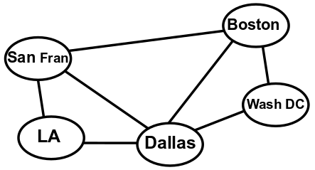
Likewise, undirected graphs are not drawn with arrowheads. The lack of arrowheads imply that the edges are two-way streets, meaning valid paths can go in either direction between vertices. They are connected (not "strongly connected") if an undirected path exists in the graph between every pair of vertices in the graph.
Graphs can represent a huge range of phenomena. For instance a graph could represent a simple road map of highways between major US cities.
Or a graph may represent the outcomes of a series of actions. This graph denotes the operations that can be performed to stack three blocks, A, B and C.
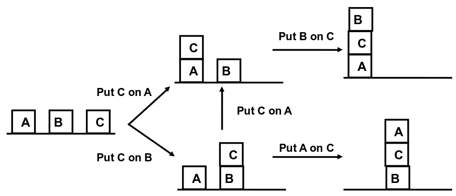
Let's think about what these graphs are telling us.
A graph is complete if all pairs of vertices in the graph appear as edges, that is, all vertices are adjacent.
One graph is a subgraph of another graph if it contains a subset of the vertices and edges of the second graph. A subgraph of an undirected graph is called a clique if it denotes a complete graph, that is, all its vertices are adjacent.
Describing Vertices
We can also describe individual vertices. The degree of a vertex is the number of edges that impinge upon that vertex. Vertices in both directed and undirected graphs have degrees.
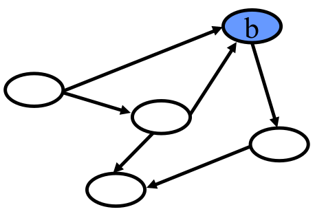
For instance, the vertex in this directed graph has two edges pointed to it and one edge pointed away. It has an in degree of 2 and and out degree of 1.
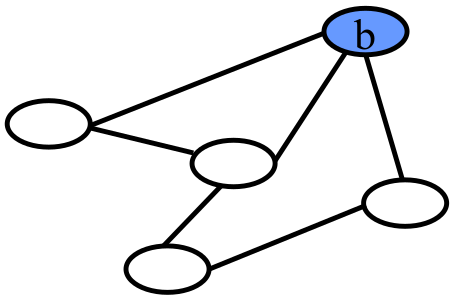
In the undirected version of the same graph, simply has a degree of 3 because of the three edges connected to it.
Specifying Graphs
The last thing you need to know about graphs before you start writing search algorithms is how we specify them, or in other words, the mathematical language we use to describe them.
Mathematically we represent a graph with sets and sequences
We denote an unordered set of elements starting with and and going through , by . Each element listed in the set is distinguished, that is, an element is not listed more than once. The idea that sets are unordered means that the set is equivalent to .
Sequences are also called lists. Lists are ordered. The notation for paths we already saw, eg. , represents an ordered list of elements starting with and and going through . The idea that a list is ordered means that is not equivalent to .
A pair is a list of two elements, a triple is a list of three, and an -tuple is a list of elements.
Putting it all togther, we represent a directed graph by a pair, whose first element is a set of vertices and whose second element is a set of edges. Each directed edge is represented by a pair, whose first element is the edge's head (where the arrow starts), and second element is the edge's tail (where the arrow ends).
Let's look at this definition in practice with the following directed graph.

The set of vertics, , is the unordered set .
The set of edges, , consists of all the pairs representing the graph's directed edges. Looking at the graph, we can see five arrows, so should be comprised of five pairs.
The entire graph is defined as a pair of the vertices and edges, .
Note that it is perfectly acceptable to nest sequences and sets. You can have a set of sequences or a sequence of sets, or sets of sets of sequences, or any combination thereof.
Let's think about the difference between how we define directed and undirected graphs.
Search Trees
To make this approach precise we need to define search tree. A search tree is a directed graph with the property that there is unique path between every pair of vertices in the graph. More precisely, there is exactly one undirected path between each pair of vertices. We accomplish this by limiting the in degree of each vertex in the tree to be at most one.
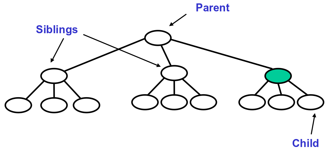
The terminology for elements of a search tree are adopted from that of a "family" tree. A family tree is a tree that grows from top to bottom. The top is a single vertex, called the root. The bottom of the tree is a set of vertices with no out degree, which are called leaves. The edges of the tree are called branches, and the vertices of the tree are called nodes.
If we look at the path from the root to vertex , the vertices along this path ( except for ) are called 's ancestors.
Conversely, every vertex along a path from to a leaf in the tree is a descendant of .
Uninformed Search
Next, we turn to the problem of defining a search algorithm that solves a state space search problem. To do so we enumerate a candidate space of partial paths that start at and we test each candidate to see if it is (1) simple and (2) ends at the goal . By simple, we mean there are no loops, ie. vertices only appear in at most once.
We would like to represent this candidate space compactly. To do so we note that all these candidate paths share the start vertex in common, and many paths share a prefix. Hence, we can represent the candidate set compactly using a tree, called a search tree. A candidate path is then a path through the tree from its top (root) to one of its bottom vertices (leaves).

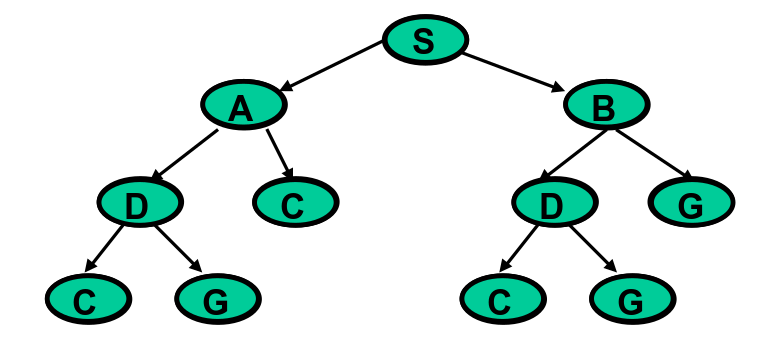
In this example, the search tree is on the right. It enumates the paths we can take from each vertex, starting from and going to until we find the solution, . The representation is partial, however. For instance, it does not enumerate any paths from to .
The full search tree starting from is as follows.

This tree represents all paths starting from and going to the leaves of the tree.
Given a precise statement of a state space search problem, we can design algorithms to solve it. The algorithm varies depending on additional features of the problem and its solution. There are many classes of search problems. These are divided into algorithms that generate all simple paths, and algorithms that focus on finding the shortest simple paths.
Algorithms that find any simple path are called "blind" or uninformed search algorithms. They are uninformed in the sense that they ignore path length. Algorithms that find the shortest paths are called optimal, or informed, algorithms. We'll have lessons on informed search algorithms for you later.
We imagine the space of possible solutions to a problem with a search tree. The nodes of the tree are states in . The tree is rooted in the start state . For every parent / child pair of nodes, there is an edge in the search problem between the corresponding states. We look are looking for leaves in the tree that contain the goal state . A solution is then a path from the root to the leaf containing .
A search algorithm explores the search tree in a particular order. To illustrate this process, I'll give you the intuition behind two uninformed search algorithms, depth-first and breadth-first search, using search trees.
For the following examples and walkthrough, we'll use the search tree below. We'll be starting at the root node, .
Depth-First Search
We can think of search algorithms as navigating a search tree in particular order. This order is defined by a set of local rules. In depth-first search (DFS), the search algorithm generates candidate paths by trying to go as deeply in the tree as can be reached, and only backing up whenever it can't explore further. We will assume that the algorithm explores the tree from left to right.
We can capture this behavior through two rules.
- Given a vertex that the search algorithm has reached, the first rule says to visit each child of first, before vising any sibling of . This causes the algorithm to push deeper.
- When at vertex , visit its children from left to right. This has the effect of exploring the search tree from the left-hand side to the right-hand side.
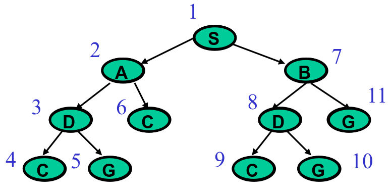
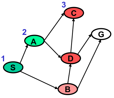
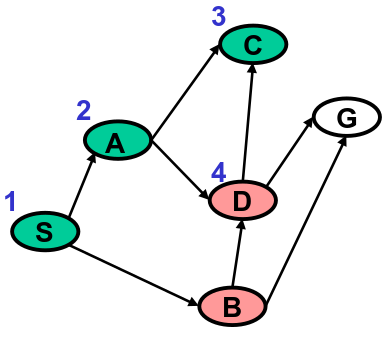
Applying the two rules yields a search that traverses the tree in the order you see in the numbers above. It starts at , then goes as far down the left side as possible, visiting , then , then . From there, it snakes to the right nodes, and , back up, and over to the right side of the tree.
We haven't walked through the complete algorithm yet, but I want you to build an intuition of how DFS works. Try the following question. Use the example DFS search tree above as a guide.
Just because building a Lego car with DFS probably isn't the best idea, doesn't mean that DFS never makes sense. There are other scenarios where it is useful. Thinking back to the block stacking graph, what if your goal was to find a set of actions to make a stack of three blocks in any order? DFS would work great then.
Breadth-First Search
Breadth-first search (BFS) enumerates candidate paths along an even front. It first enumerates all paths with one edge, then two edges, then three edges and so forth.
It accomplishes this with two local rules.
- Unlike DFS, visit all siblings of the current visited node before visiting any of its children. The net affect is to spread enumeration wide rather than deep.
- Like DFS, order enumeration so that paths are generated from left to right in the tree.

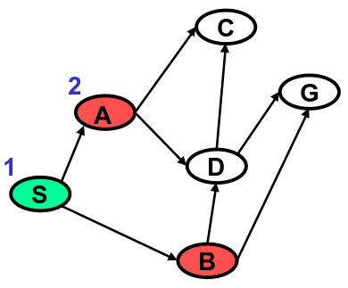
Starting at , the first rule has the effect of visiting all of its children, and , before traversing deeper down the tree.
If you've been answering all the questions so far, you've been thinking a lot about systematically building Legos. It should be clear that neither DFS nor BFS is the most effective search algorithm, broadly speaking. Rather, they are extremely useful to learn because they form the backbone of a wide range of search algorithms with real-world applications that we'll be exploring later on.
With DFS and BFS in hand, you're almost ready to implement a solution to solve a search problem. But first, we a detailed look at the algorithm for state space search.
State Space Search Walkthrough
Recall that a state space search problem consists of a set of states, which describe where we are in the search, and operators, which describe how to move between states. Our search state keeps track of the candidates that still need to be enumerated. The operator generates candidates, checks if they are solutions, and returns an updated search state.
How do we maintain search state? The basic operation of search is to extend partial paths, beginning at . In this case, partial refers to the fact that the paths do not include the goal. Extensions refer to growing a path by following the search tree.
For example, suppose that path from the graph above is expanded. has two children, and . The expansion produces two new partial paths that extend to its children, creating and .
In order to perform search we must maintain a set of partial paths that are yet to be expanded. We call this a queue, . We start with the search state , where is a partial path that is the beginning of all valid solutions (you must start at !). As search is performed, partial paths are added to this queue. We will see an example in a moment.
The basic operation that search performs takes a search state as input and returns an updated search state. It should also terminate when search is complete. To do so, the operation removes some path from , expands and adds all expansions to . If ends at the goal, , then the operator returns as a solution. If is empty, then no candidates remain, and the operator terminates search with no solution.
At a high-level, state space search:
- Maintains a queue, , which is a list of partial paths it has not expanded yet
- Repeatedly performs the following operations:
- Selects a partial path, , from
- Expands by following the edges on the search tree
- Adds expansions to
- Terminates when the goal, , is found, or when is empty
There are a few edge cases for search we haven't covered yet.
State space search is complete, that is, the algorithm always finds a solution if one exists. We can also say the algorithm is systematic because it never expands a candidate path twice.
One last note before we look at the full algorithm. We'll store paths in reverse order, eg. instead of representing a partial path, we'll store it as . This simplifies looking up the last visited node of the list because it is always the head. We will use the head(P) operator to represent the first node in .
Simple Search Algorithm Pseudocode
Let be a list of partial paths
Let be the start node
Let be the goal node
- Initialize the queue with the start node
- If is empty: return
fail - Else, pick a partial path from
- If
head(N)is , return as the solution - Else
- Remove from
- Find all children of
head(N) - For each child, create a one-step extension of to the child
- Add all expansions to
GOTOstep 2
Steps 2 and 4 check if we have exhausted our search or if the goal has been reached. Steps 5.2 and 5.3 are the expansion process described before.
DFS Walkthrough
We'll now walk through an implementation of DFS on the search tree seen above. We'll use a table to represent at each iteration.
Iteration 1
is initialized to .
| Iteration | Queue |
|---|---|
| 1 | S |
| 2 | |
| 3 | |
| 4 | |
| 5 | |
| 6 |
The queue is not empty, so we execute step 3. The only path is . head(N) is not , so we execute step 5
For step 5.1, we remove from .
| Iteration | Queue |
|---|---|
| 1 | |
| 2 | |
| 3 | |
| 4 | |
| 5 | |
| 6 |
The strikethrough of means that it has been removed from .
For step 5.2, we find and are the children of . For step 5.3, we create and (remember, partial paths are backwards so we can use the head operator).
For step 5.4, we add the extensions to . According to DFS we should add partial paths to in the order they appear from left to right. Our graph is skewed sideways, so we'll add them to from top to bottom.
| Iteration | Queue |
|---|---|
| 1 | |
| 2 | AS, BS |
| 3 | |
| 4 | |
| 5 | |
| 6 |
Then we go back to step 2 and begin a new iteration.
Iteration 2
Green means the node has already been visited. Red nodes are the heads of paths that have been newly added to .
is not empty, so we execute step 3. We pop the first path off , . head(N) is not , so we execute step 5.
For step 5.1, we remove from .
| Iteration | Queue |
|---|---|
| 1 | |
| 2 | |
| 3 | |
| 4 | |
| 5 | |
| 6 |
has children and . For step 5.3, we create and .
For step 5.4, we add the expansions of to the head of . Remember, DFS searches children before siblings. We want the path expansions of , and , to be popped off the head of the queue before its sibling, .
| Iteration | Queue |
|---|---|
| 1 | |
| 2 | |
| 3 | CAS, DAS, BS |
| 4 | |
| 5 | |
| 6 |
Once again, we go back to step 2 and begin a new iteration.
Iteration 3
Light red represents a node that is one the queue but has not been expanded. Light green represents a node that is still on the queue and it has been expanded.
For step 3, we pick from the head of . head(N) is not , so we continue to step 5 and pop off .
| Iteration | Queue |
|---|---|
| 1 | |
| 2 | |
| 3 | |
| 4 | |
| 5 | |
| 6 |
head(N) is . There are no children of , so we cannot execute steps 5.2, 5.3, or 5.4. We move on to the next iteration.
Iteration 4
| Iteration | Queue |
|---|---|
| 1 | |
| 2 | |
| 3 | |
| 4 | DAS, BS |
| 5 | |
| 6 |
For step 3, we pick from the head of . head(N) is not , so we continue to step 5 and pop off .
| Iteration | Queue |
|---|---|
| 1 | |
| 2 | |
| 3 | |
| 4 | |
| 5 |
has two children, and . For steps 5.2, 5.3, and 5.4, we add and to Q.
| Iteration | Queue |
|---|---|
| 1 | |
| 2 | |
| 3 | |
| 4 | |
| 5 | CDAS, GDAS, BS |
| 6 |
We then move on to the next iteration.
Iteration 5
It's your turn. Don't scroll down yet! Instead, walk through the algorithm yourself for this iteration.
Iteration 6
Did you answer the question above yet? If not, do it now!
| Iteration | Queue |
|---|---|
| 1 | |
| 2 | |
| 3 | |
| 4 | |
| 5 | |
| 6 | GDAS, BS |
For step 2, is not empty. For step 3, we pick . For step 4, we find that head(N) is ! We return . With that, the algorithm stops and we've finished this walkthrough.
Implementing BFS vs DFS
Remember that BFS differs from DFS in that we generally want to explore siblings before children. The overall algorithm for BFS is almost exactly the same as we just saw for DFS, with only one difference.
It is time to write some code! You'll implement both DFS and BFS to solve a new problem.
Decision Making: Solving an 8-Tile Puzzle
As a simple example of a state space search problem, we consider the 8-Tile Puzzle. Most of us are familiar with this puzzle from our childhood. We are given the tile puzzle in some start configuration and are challenged to move the tiles until the puzzle reaches a specified goal configuration. Start and Goal configurations are shown to the left and to the right below.
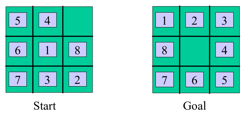
States: Integer locations for all tiles (can you think of anything else?)
Operators: Move empty square up, down, left, right
Initial and Goal States: See above
We frame the 8-Puzzle as a state space search problem by defining a set of states, a set of operators for moving between states, the initial state, and the goal state. The state space is the set of possible configurations of the 8-Tile Puzzle, that is to say, the possible placements of tiles.
The size and simplicity of the state and operator encoding can have a dramatic impact on the efficiency of the problem solver. In this example, one way of encoding a state (configuration) is to associate a variable with each tile 1-8. and assign each of these tile variables an integer, 1-9, denoting the tiles position in a particular configuration. We number positions from left to right and top to bottom. We note that one position in a configuration is always empty. We will treat the “empty square” as if it is another tile and assign it an integer position as well.
The reason to give the empty square a position is that it will make it easy to describe the problem’s operator. The operator involves moving a tile into an adjacent empty square. We can equivalently view this operation as moving the empty square to a neighboring position. From this perspective, the empty square can move up, down, left or right, and has the effect of swapping positions with the tile that it overtakes. Given this encoding, the initial and goal states are specified as integer assignments to tile variables that correspond to the pictures above.
Python Implementation
Are you ready to try solving this problem? Here's a link to a Jupyter notebook where you can put your Python skills to the test: link.